Presenting the Calendar! 📅
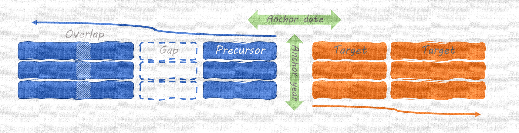
To explain some of the terminology used in this package, the image below can be used as reference.
The calendar system revolves around so-called “anchor dates” and “anchor years”. The anchor date is (generally) the start of the period you want to forecast. I.e. your target data. The anchor date is an abstract date, and does not include a year. For example, 5 June, or 25 December 🎄.
Anchor years are used to create a full date with the anchor date (e.g., 25 December 2022), and to group the calendar intervals together.
Two types of intervals exist. First are the target intervals, which is generally what you want to predict or forecast. The other type are precursor intervals, intervals preceding the anchor date representing the data that you would like to use to forecast the target interval.
Using the calendar
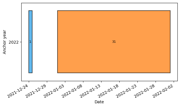
First we import the package, and create an empty calendar with the anchor date 25 December:
[1]:
from lilio import Calendar
cal = Calendar("12-25")  # 🎄🎅
cal
[1]:
Calendar(
    anchor='12-25',
    allow_overlap=False,
    mapping=None,
    intervals=None
)
To this calendar we can add an interval, in this case a “target” interval which we want to use as our target data.
Note that when calling add_intervals, the default n (number of intervals) is 1.
[2]:
cal.add_intervals("target", length="1d")
When viewing the calendar, you can see that the calendar now contains this interval
[3]:
cal
[3]:
Calendar(
    anchor='12-25',
    allow_overlap=False,
    mapping=None,
    intervals=[
        Interval(role='target', length='1d', gap='0d')
    ]
)
However, this calendar is not mapped to any years yet. Before we can view which dates are represented by each interval, we have to map the calendar:
[4]:
cal.map_years(start=2021, end=2022)
[4]:
Calendar(
    anchor='12-25',
    allow_overlap=False,
    mapping=('years', 2021, 2022),
    intervals=[
        Interval(role='target', length='1d', gap='0d')
    ]
)
Now we can call .show() and view the intervals generated. A table is returned, showing the anchor year(s) on the vertical axis and the intervals on the horizontal index, sorted by their interval index (i_interval).
[5]:
cal.show()
[5]:
| i_interval | 1 |
|---|---|
| anchor_year | |
| 2022 | [2022-12-25, 2022-12-26) |
| 2021 | [2021-12-25, 2021-12-26) |
We can add some precursor periods, and inspect the table again. We can add multiple intervals using the n keyword argument.
Note that the target interval has a positive index, while the precursors have negative indices.
[6]:
cal.add_intervals("precursor", length="1d", n=6)
cal.show()
[6]:
| i_interval | -6 | -5 | -4 | -3 | -2 | -1 | 1 |
|---|---|---|---|---|---|---|---|
| anchor_year | |||||||
| 2022 | [2022-12-19, 2022-12-20) | [2022-12-20, 2022-12-21) | [2022-12-21, 2022-12-22) | [2022-12-22, 2022-12-23) | [2022-12-23, 2022-12-24) | [2022-12-24, 2022-12-25) | [2022-12-25, 2022-12-26) |
| 2021 | [2021-12-19, 2021-12-20) | [2021-12-20, 2021-12-21) | [2021-12-21, 2021-12-22) | [2021-12-22, 2021-12-23) | [2021-12-23, 2021-12-24) | [2021-12-24, 2021-12-25) | [2021-12-25, 2021-12-26) |
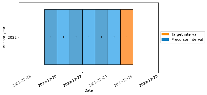
Besides a table view, the calendar can also be visualized in a plot. The default plotting backend is matplotlib (as in the image below).
An interactive ‘bokeh’ plot, containing more information on the intervals, is also available. It is used by calling .visualize(interactive=True). Do note that bokeh needs to be installed for this to work.
[7]:
cal.visualize(n_years=1, add_legend=True, show_length=True)
For inputs such as length, you can use either days ("10d"), weeks ("3W") or months ("1M").
[8]:
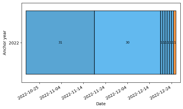
cal.add_intervals("precursor", length="1M", n=2)
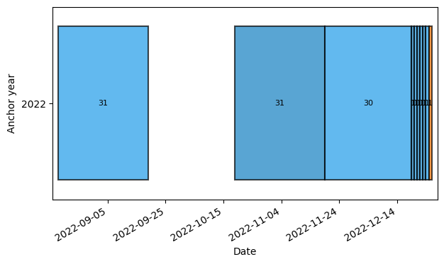
Note that in the visualization below, the length of the large precursor blocks is 31 and 30 days respectively, this is due to the input length of 1M, and the months not having the same lengths
[9]:
cal.visualize(n_years=1, add_legend=False, show_length=True)
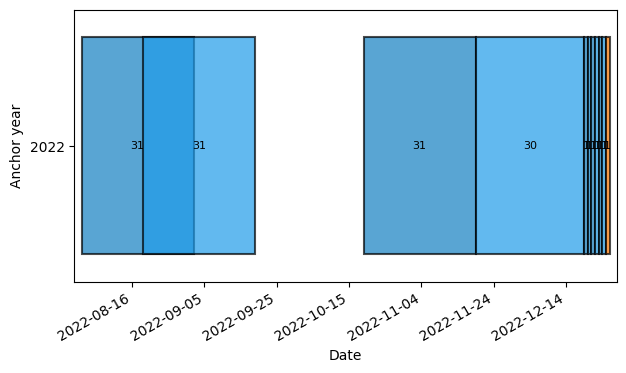
Last but not least, are gaps. Gaps can be inserted between the previous interval and the new one:
[10]:
cal.add_intervals("precursor", length="1M", gap="1M")
cal.visualize(n_years=1, add_legend=False, show_length=True)
Note that these gaps can also be negative. This makes the new interval overlap with the previous one.
[11]:
cal.add_intervals("precursor", length="1M", gap="-2W")
cal.visualize(n_years=1, add_legend=False, show_length=True)
Using the “repr” to reproduce calendars 📜
When you just call the calendar, as in the cell below, the calendar will return a string representation of itself. This is enough information to completely rebuild the calendar, so it can be used as a way to store or share a specific calendar.
[12]:
cal = Calendar("06-01")
cal.map_years(2020, 2022)
cal.add_intervals("target", "1d")
cal.add_intervals("precursor", "7d", "1M")
cal
[12]:
Calendar(
    anchor='06-01',
    allow_overlap=False,
    mapping=('years', 2020, 2022),
    intervals=[
        Interval(role='target', length='1d', gap='0d'),
        Interval(role='precursor', length='7d', gap='1M')
    ]
)
Here we copy-paste the calendar, and we import the required classes from lilio. Note that it reproduces itself when you call cal
[13]:
from lilio import Interval
Calendar(
    anchor='06-01',
    allow_overlap=False,
    mapping=('years', 2020, 2022),
    intervals=[
        Interval(role='target', length='1d', gap='0d'),
        Interval(role='precursor', length='7d', gap='1M')
    ]
)
cal
[13]:
Calendar(
    anchor='06-01',
    allow_overlap=False,
    mapping=('years', 2020, 2022),
    intervals=[
        Interval(role='target', length='1d', gap='0d'),
        Interval(role='precursor', length='7d', gap='1M')
    ]
)
The Interval building block 🧱
The basic building block of the Calendar is the Interval. Intervals have three properties: the type (target or precursor), the length, and the gap. The gap is defined as the gap between this interval and the preceding interval of the same type (or the anchor, if this interval is the first one).
The length and gap are set in the same way. The most common way is to use a pandas-like frequency string (for example, “10d” for ten days, “2W” for two weeks, or “3M” for three months). Let’s set the length to five days and the gap to a month:
[14]:
iv = Interval("target", length="5d", gap="1M")
iv
[14]:
Interval(role='target', length='5d', gap='1M')
Intervals can be changed in-place. Their gap and length can be set in the following way:
[15]:
iv.gap = "5d"
iv
[15]:
Interval(role='target', length='5d', gap='5d')
If you are feeling adventurous, you can set the length and gap using a pandas.DateOffset compatible dictionary. This allows you to combine day, week, and month lengths:
[16]:
iv.length = {"months": 1, "weeks": 2}
iv.length_dateoffset  # shows the length as a pandas.DateOffset object.
[16]:
<DateOffset: months=1, weeks=2>
All about anchors ⚓
As said before, the anchor date is one of the basic elements of the calendar. Up to now we have just showcased setting the anchor as a date (“MM-DD”), however, there are some alternative options.
If you are interested in only months, it is possible to create a calendar revolving solely around calendar months. The anchor can be defined as an English month name (e.g., “January” or the short name “Jan”). This is equivalent to setting the anchor to the first day of that month. For example:
[17]:
cal = Calendar(anchor="December")  # [December 01)
cal.add_intervals("target", "1M")
cal.add_intervals("precursor", "1M", n=11)
cal.map_years(2022, 2022)
cal.show()
[17]:
| i_interval | -11 | -10 | -9 | -8 | -7 | -6 | -5 | -4 | -3 | -2 | -1 | 1 |
|---|---|---|---|---|---|---|---|---|---|---|---|---|
| anchor_year | ||||||||||||
| 2022 | [2022-01-01, 2022-02-01) | [2022-02-01, 2022-03-01) | [2022-03-01, 2022-04-01) | [2022-04-01, 2022-05-01) | [2022-05-01, 2022-06-01) | [2022-06-01, 2022-07-01) | [2022-07-01, 2022-08-01) | [2022-08-01, 2022-09-01) | [2022-09-01, 2022-10-01) | [2022-10-01, 2022-11-01) | [2022-11-01, 2022-12-01) | [2022-12-01, 2023-01-01) |
Besides months, the calendar can also be used with week numbers. You can use either only a week number (“W10” for the 10th week of a year), or the combination of a week number and the day of the week (where Monday is 1 and Sunday 7). This can be especially useful with targets and precursor intervals that you would like to cover certain days of the week. For example:
[18]:
Calendar(anchor="W12")  # Week 12
cal = Calendar(anchor="W12-5")  # Friday on week 12
cal.add_intervals("target", "1d")
cal.add_intervals("precursor", "1d", gap="1W")
cal.map_years(2018, 2022)
cal.show()
[18]:
| i_interval | -1 | 1 |
|---|---|---|
| anchor_year | ||
| 2022 | [2022-03-17, 2022-03-18) | [2022-03-25, 2022-03-26) |
| 2021 | [2021-03-18, 2021-03-19) | [2021-03-26, 2021-03-27) |
| 2020 | [2020-03-19, 2020-03-20) | [2020-03-27, 2020-03-28) |
| 2019 | [2019-03-21, 2019-03-22) | [2019-03-29, 2019-03-30) |
| 2018 | [2018-03-15, 2018-03-16) | [2018-03-23, 2018-03-24) |
Modifying calendars in-place 🏗️
If you want to do funkier things with the calendar, you can edit already existing calendars 🔨👷♀️
For example, the anchor of the calendar can be changed:
[19]:
cal.anchor = "01-01"  # 🍾🥂
cal
[19]:
Calendar(
    anchor='01-01',
    allow_overlap=False,
    mapping=('years', 2018, 2022),
    intervals=[
        Interval(role='target', length='1d', gap='0d'),
        Interval(role='precursor', length='1d', gap='1W')
    ]
)
In this case, you do need to be careful when comparing two calendars, as data might have shifted to a different anchor year.
Modifying the intervals is also possible. The precursors and target intervals are stored in lists, and can be changed in-place:
[20]:
cal.precursors # or cal.targets
[20]:
[Interval(role='precursor', length='1d', gap='1W')]
Now let’s change the gaps and lengths (for sake of demonstration):
[21]:
for precursor in cal.precursors:
    precursor.gap = "7d"

for target in cal.targets:
    target.length="1M"

cal.map_years(2022, 2022)
cal.visualize(add_legend=False, show_length=True)
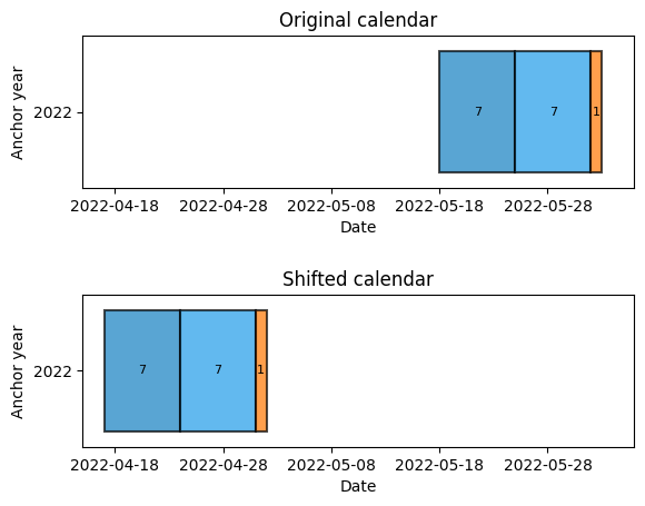
A more useful trick can be modifying the gap property of only the first target and precursor intervals. This allows you to shift all intervals relative to the anchor date.
This shifting is demonstrated below:
[22]:
import matplotlib.pyplot as plt
import numpy as np

cal = Calendar(
    anchor='06-01',
    allow_overlap=False,
    mapping=('years', 2020, 2022),
    intervals=[
        Interval(role='target', length='1d', gap='0d'),
        Interval(role='precursor', length='7d', gap='0d'),
        Interval(role='precursor', length='7d', gap='0d')
    ]
)

fig, (ax1, ax2) = plt.subplots(nrows=2)
# Plot the original calendar
cal.visualize(n_years=1, add_legend=False, show_length=True, ax=ax1)

# Shift the calendar by a month
cal.precursors[0].gap = "1M"
cal.targets[0].gap = "-1M"

# Plot the shifted calendar
cal.visualize(n_years=1, add_legend=False, show_length=True, ax=ax2)

# Make the plot pretty
ax1.set_title("Original calendar")
ax2.set_title("Shifted calendar")
for ax in (ax1, ax2):
    ax.set_xlim((np.datetime64("2022-04-15"), np.datetime64("2022-06-05")))
fig.subplots_adjust(hspace=0.7)